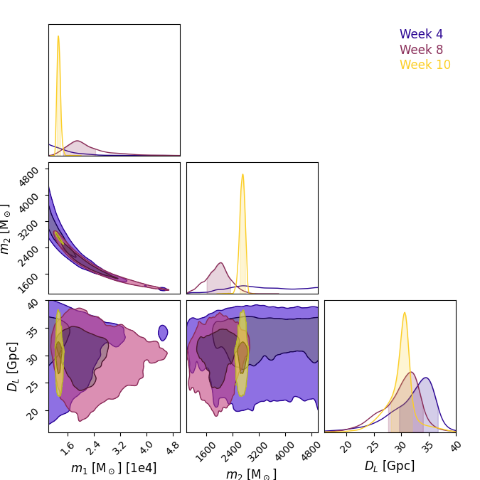
Time-evolving parameter estimation

Corner plot of select parameters for a single source showing how parameter estimation changes with observing time.

import matplotlib.pyplot as plt
from chainconsumer import ChainConsumer

from lisacattools.catalog import GWCatalogs
from lisacattools.catalog import GWCatalogType


# Find the list of catalogs
catPath = "../../tutorial/data/mbh"
catalogs = GWCatalogs.create(GWCatalogType.MBH, catPath, "*.h5")

last_cat = catalogs.get_last_catalog()
detections_attr = last_cat.get_attr_detections()
detections = last_cat.get_detections(detections_attr)

Choose a source from the list of detections and get its history through the different catalogs Pick a source, any source

sourceIdx = "MBH005546845"

Load chains for different observing epochs of selected source Get source history and display table with parameters and observing weeks containing source

srcHist = catalogs.get_lineage(last_cat.name, sourceIdx)
srcHist.drop_duplicates(subset="Log Likelihood", keep="last", inplace=True)
srcHist.sort_values(by="Observation Week", ascending=True, inplace=True)
srcHist[
    [
        "Observation Week",
        "Parent",
        "Log Likelihood",
        "Mass 1",
        "Mass 2",
        "Luminosity Distance",
    ]
]

# Load chains for different observing epochs of selected source
allEpochs = catalogs.get_lineage_data(srcHist)

Create corner for multiple observing epochs

# Choose weeks for plot from source history table
wks = [4, 8, 10]

# select subset of parameters to plot
parameters = ["Mass 1", "Mass 2", "Luminosity Distance"]
parameter_labels = [
    r"$m_1\ [{\rm M}_\odot]$",
    r"$m_2\ [{\rm M}_\odot]$",
    r"$D_L\ [{\rm Gpc}]$",
]
ranges = [(10000, 50000), (1000, 5000), (16, 40)]

c = ChainConsumer()
for idx, wk in enumerate(wks):
    epoch = allEpochs[allEpochs["Observation Week"] == wk]
    samples = epoch[parameters].values
    c.add_chain(samples, parameters=parameter_labels, name="Week " + str(wk))

c.configure(cmap="plasma")
fig = c.plotter.plot(figsize=1.5, log_scales=False, extents=ranges)
plt.show()