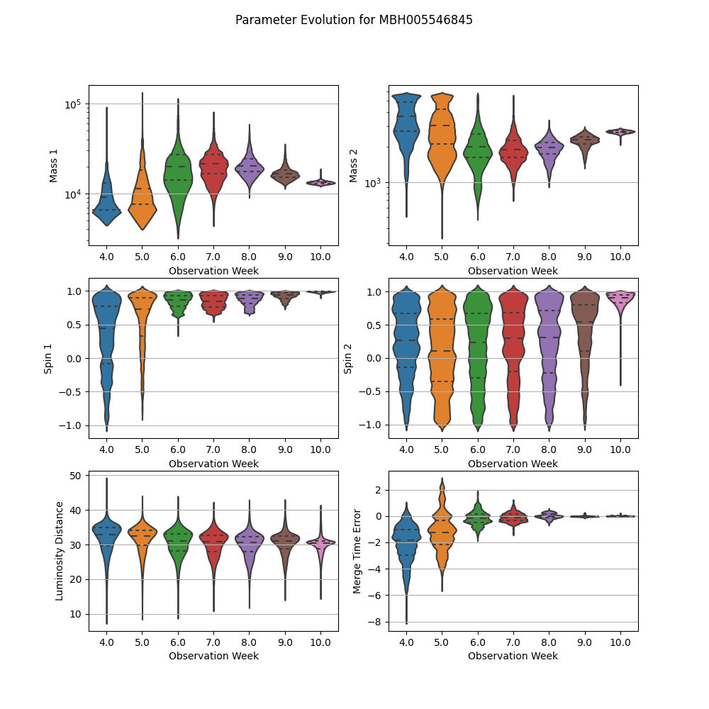
Time-evolving violin plot

Violin plot of select parameters for a single source showing how parameter estimation changes with observing time over all observing epochs

import matplotlib.pyplot as plt
import numpy as np
import seaborn as sns

from lisacattools.catalog import GWCatalogs
from lisacattools.catalog import GWCatalogType

# get list catalog files
catPath = "../../tutorial/data/mbh"
catalogs = GWCatalogs.create(GWCatalogType.MBH, catPath, "*.h5")

last_cat = catalogs.get_last_catalog()
detections_attr = last_cat.get_attr_detections()
detections = last_cat.get_detections(detections_attr)

detections = detections.sort_values(by="Mass 1")
detections[
    ["Parent", "Log Likelihood", "Mass 1", "Mass 2", "Luminosity Distance"]
]

	Parent	Log Likelihood	Mass 1	Mass 2	Luminosity Distance
name
MBH010993271	MBH010993145	58.644439	6043.582334	1484.773218	22.671702
MBH006058694	MBH006058694	119.338404	10349.085349	3303.282920	47.235091
MBH000373540		60.282950	11191.400618	1573.347120	22.205113
MBH002301433		67.615841	12659.907280	3912.600441	34.400859
MBH005546845	MBH005546845	652.996924	13238.473697	2707.606755	30.323258
MBH004556400	MBH004556400	243.337498	15868.967713	9036.333963	28.921349
MBH004650719	MBH004650719	446.562104	22450.923508	8796.170612	59.148264
MBH001865195	MBH001865195	164.506458	24034.822836	8748.509775	95.079793
MBH007449510	MBH007449510	72.207804	38276.504295	2615.575967	100.930430
MBH006253789	MBH006253789	260.016246	51499.191655	5166.812496	24.506354
MBH011318669	MBH011317078	740.270521	142698.356416	31498.663144	13.886229
MBH007807200	MBH007807200	189597.629550	641359.177017	83719.952286	14.897055

Choose a source from the list of detections and get its history through the different catalogs

# Pick a source, any source
sourceIdx = "MBH005546845"

# Get source history and display table with parameters and observing weeks containing source
srcHist = catalogs.get_lineage(last_cat.name, sourceIdx)
srcHist.drop_duplicates(subset="Log Likelihood", keep="last", inplace=True)
srcHist.sort_values(by="Observation Week", ascending=True, inplace=True)
srcHist[
    [
        "Observation Week",
        "Parent",
        "Log Likelihood",
        "Mass 1",
        "Mass 2",
        "Luminosity Distance",
    ]
]

allEpochs = catalogs.get_lineage_data(srcHist)

# For plotting purposes, we add a new parameter that is merger time error (in hours), expressed relative to median merger time after observation is complete
latestWeek = np.max(allEpochs["Observation Week"])
allEpochs["Merge Time Error"] = (
    allEpochs["Barycenter Merge Time"]
    - np.median(
        allEpochs[allEpochs["Observation Week"] == latestWeek][
            "Barycenter Merge Time"
        ]
    )
) / 3600

Create the violin plot select the parameters to plot and scaling (linear or log) for each

params = [
    "Mass 1",
    "Mass 2",
    "Spin 1",
    "Spin 2",
    "Luminosity Distance",
    "Merge Time Error",
]
scales = ["log", "log", "linear", "linear", "linear", "linear"]

# arrange the plots into a grid of subplots
ncols = 2
nrows = int(np.ceil(len(params) / ncols))
fig = plt.figure(figsize=[10, 10], dpi=100)

# plot the violin plot for each parameter
for idx, param in enumerate(params):
    ax = fig.add_subplot(nrows, ncols, idx + 1)
    sns.violinplot(
        ax=ax,
        x="Observation Week",
        y=param,
        data=allEpochs,
        scale="width",
        width=0.8,
        inner="quartile",
    )
    ax.set_yscale(scales[idx])
    ax.grid(axis="y")

# add an overall title
fig.suptitle("Parameter Evolution for %s" % sourceIdx)
plt.show()