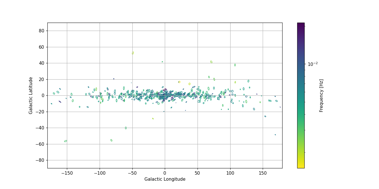
Sky Localization Ellipses

Plot 1-sigma contours of well-localized sources’ sky location in galactic coordinates.

Load catalog and compute sky areas

import matplotlib.cm as cm
import matplotlib.colors as colors
import matplotlib.pyplot as plt
import numpy as np
import pandas as pd
from matplotlib.patches import Ellipse

from lisacattools import confidence_ellipse
from lisacattools import convert_ecliptic_to_galactic
from lisacattools import ellipse_area
from lisacattools import GWCatalog
from lisacattools import GWCatalogs
from lisacattools import GWCatalogType

# Start by loading the main catalog file processed from GBMCMC outputs
catPath = "../../tutorial/data/ucb"
catalogs = GWCatalogs.create(GWCatalogType.UCB, catPath, "cat15728640_v2.h5")
final_catalog = catalogs.get_last_catalog()
detections_attr = final_catalog.get_attr_detections()
detections = final_catalog.get_detections(detections_attr)


# loop through all of the sources, compute sky area, and add as a column to the catalog
area = np.empty(len(detections.index))

sources = list(detections.index)
for idx, source in enumerate(sources):

    # load source chain
    samples = final_catalog.get_source_samples(source)

    # correct sign error in catalog production
    samples["Ecliptic Latitude"] = np.pi / 2 - np.arccos(samples["coslat"])

    # convert from ecliptic to galactic coordinates
    convert_ecliptic_to_galactic(samples)

    # create numpy arrays of the derived parameters
    area[idx] = ellipse_area(
        samples[["Galactic Longitude", "Galactic Latitude"]]
    )

# insert new numpy arrays into main catalog dataframe
detections.insert(len(detections.columns), "Sky Area", area, True)

# show that, indeed, Sky Area is now a column in the dataframe
detections[["Frequency", "SNR", "Sky Area"]].head()

	Frequency	SNR	Sky Area
name
LDC0081497609	0.008150	30.9800	326.231661
LDC0081535331	0.008154	19.2096	541.571806
LDC0081547837	0.008155	148.8680	11.854226
LDC0081595365	0.008160	88.8300	69.814925
LDC0081697901	0.008170	19.8016	854.075802

Cut source catalog on localization, and plot skymap of selected sources. In this example we use 100 sq deg as the localization threshold. NOTE: 10 sq deg is more appropriate for EM follow-up, but makes for a less interesting figure

# Make new dataframe containing only "well-localized" events
max_sky_area = 100  # localization threshold (square degrees)
cat_loc = detections[
    (detections["Sky Area"] < max_sky_area)
]  # cut sources based on max_sky_area

# set up the figure
fig = plt.figure(figsize=(12, 6), dpi=110)
ax = plt.axes()

ax.grid()
ax.set(
    xlim=(-180, 180),
    ylim=(-90, 90),
    xlabel="Galactic Longitude",
    ylabel="Galactic Latitude",
)

# color ellipses by log frequency
cNorm = colors.LogNorm(
    vmin=cat_loc["Frequency"].min(), vmax=cat_loc["Frequency"].max()
)
scalarMap = cm.ScalarMappable(norm=cNorm, cmap=plt.cm.get_cmap("viridis_r"))
cbar = fig.colorbar(scalarMap)
cbar.set_label("Frequency [Hz]")

# loop over all sources adding ellipse to plot
sources = list(cat_loc.index)
for source in sources:

    # get chain samples
    samples = final_catalog.get_source_samples(source)

    samples["Ecliptic Latitude"] = np.pi / 2 - np.arccos(samples["coslat"])

    # convert from ecliptic to galactic coordinates
    convert_ecliptic_to_galactic(samples)

    # get centroid and 1-sigma contours in galactic coordinates, add to plot
    confidence_ellipse(
        samples[["Galactic Longitude", "Galactic Latitude"]],
        ax,
        n_std=1.0,
        edgecolor=scalarMap.to_rgba(np.array(cat_loc.loc[source].Frequency)),
        linewidth=1.0,
    )

plt.show()

Out:

/home/runner/work/lisacattools/lisacattools/docs/examples_ucb/plot_source_sky_ellipses.py:87: MatplotlibDeprecationWarning: Unable to determine Axes to steal space for Colorbar. Using gca(), but will raise in the future. Either provide the *cax* argument to use as the Axes for the Colorbar, provide the *ax* argument to steal space from it, or add *mappable* to an Axes.
  cbar = fig.colorbar(scalarMap)